Intro_FindIT2:integrate_ChIP_RNA module
在上一篇介绍calcRP module的结尾,我提到了可以将calcRP_TFHit的输出结果作为integrate_ChIP_RNA函数的输入,从而来实现ChIP-seq和RNA-seq的整合。所以这篇文章我就来讲讲integrate_ChIP_RNA这个模块。
integrate_ChIP_RNA模块只有一个同名的函数integrate_ChIP_RNA,其目的就是要将ChIP-seq和RNA-seq的数据整合起来,从而更准确地寻找到TF对应的靶基因。在我看来,ChIP-seq和RNA-seq的联合分析可以互相弥补两种组学寻找TF靶基因的优缺点。首先对于RNA-seq而言,我们通过TF KO/OE得到的RNA-seq的差异基因并不一定是TF的direct target。因为生物的互作网络是一个非常复杂的结构,你对其进行扰动,受到影响的不一定只有直接关联的靶基因,很多时候一些跟你TF关联较远的基因也会受到影响。反应到RNA-seq的结果上来就是你的差异基因会非常地多。而对于ChIP-seq而言,尽管得到的是direct target site,但由于抗体、建库等客观因素的影响,很多时候做实验的体系并不一定理想体系,那么你的target寻找就有可能存在一定的bias。所以,通过将ChIP-seq和RNA-seq的结果进行整合,我们可以尽可能地在还原真实状态下的同时,又寻找到感兴趣TF的直接target基因。
尽管ChIP-seq和RNA-seq的整合有利于靶基因更加精确的寻找,但传统整合方法却非常的粗暴,就是把ChIP-seq的靶基因和RNA-seq的差异基因取一个交集。对于ChIP-seq的靶基因,一般用最近基因注释,来为每个peak找一个最近的target基因,而对于RNA-seq,则是取一个比较随意的阈值,比如abs(log2FoldChang) > 1 & padj < 0.05,来决定差异。这么做有几个缺点,首先就是最近基因注释并不一定真正能揭示peak与target的调控关系,事实上一个peak可能调控多个基因,一个基因可能也会被多个peak,又或者一个peak簇会调控一组基因。其次就是差异基因的阈值选定是很武断的,有些RNA-seq差异很大,abs(log2FoldChang) > 1 & padj < 0.05会得到很多基因,而有些RNA-seq差异较小,用这个阈值得到的基因反而很少。最后就是单纯地交集选择除了给我们一个基因list之外,并不能给我们提供额外有价值的信息。
考虑到以上的交集选择缺陷,integrate_ChIP_RNA函数使用了一种rank product的整合方法,即将ChIP-seq得到的target gene rank和RNA-seq得到的target gene rank进行乘积,如果一个基因在ChIP-seq和RNA-seq中的rank都很前面,那么最终的排名就会非常的靠前。具体的实现步骤我会通过一个例子来讲解。
Pre-preparation
这次的测试数据仍旧来自于FindIT2包本身,包含一个TF的ChIP-seq peak文件和TF受诱导的RNA-seq差异文件。
# 加载包
library(FindIT2)
library(TxDb.Athaliana.BioMart.plantsmart28)
library(ggplot2)

Txdb <- TxDb.Athaliana.BioMart.plantsmart28
seqlevels(Txdb) <- paste0("Chr", c(1:5, "M", "C"))
# 加载相关数据
ChIP_peak_path <- system.file("extdata", "ChIP.bed.gz", package = "FindIT2")
ChIP_peak_GR <- loadPeakFile(ChIP_peak_path)
# 再次说明,请有feature_id这个列名
# 如果你想要calcRP_TFHit考虑每个peak的分数,就还需要一列feature_score
ChIP_peak_GR
## GRanges object with 4288 ranges and 2 metadata columns:
## seqnames ranges strand | feature_id score
## <Rle> <IRanges> <Rle> | <character> <numeric>
## [1] Chr5 6236-6508 * | peak_14125 27
## [2] Chr5 7627-8237 * | peak_14126 51
## [3] Chr5 9730-10211 * | peak_14127 32
## [4] Chr5 12693-12867 * | peak_14128 22
## [5] Chr5 13168-14770 * | peak_14129 519
## ... ... ... ... . ... ...
## [4284] Chr5 26937822-26938526 * | peak_18408 445
## [4285] Chr5 26939152-26939267 * | peak_18409 21
## [4286] Chr5 26949581-26950335 * | peak_18410 263
## [4287] Chr5 26952230-26952558 * | peak_18411 30
## [4288] Chr5 26968877-26969091 * | peak_18412 26
## -------
## seqinfo: 1 sequence from an unspecified genome; no seqlengths
# 加载矩阵数据
data("RNADiff_LEC2_GR")
head(RNADiff_LEC2_GR)
## gene_id log2FoldChange padj
## 1 AT5G00730 NA NA
## 2 AT5G01010 -0.04782798 0.9995524
## 3 AT5G01015 -0.28867596 0.9936103
## 4 AT5G01017 NA NA
## 5 AT5G01020 -0.13143524 0.9690018
## 6 AT5G01030 -0.30567845 0.2921698ChIP-seq rank
由于我们最终的target rank由ChIP-seq和RNA-seq两部分组成,我们首先来计算ChIP-seq的rank。rank的排序依照的就是每个基因附近周围的调控潜能,换句话说,如果一个基因附近的TF ChIP-seq 的binding site越多,那么其就越有可能会是TF的target。通过calcRP_TFHit,我们就可以得到每个基因的基于TF ChIP-seq的调控潜能。
# 先用mm_geneScan得到的ChIP-seq peak跟gene TSS的距离关系
mmAnno_TFHit <- mm_geneScan(ChIP_peak_GR,
                            Txdb,
                            upstream = 2e4,
                            downstream = 2e4)
## >> checking seqlevels match...       2021-09-24 16:25:51
## >> your peak_GR seqlevel:Chr5...
## >> your Txdb seqlevel:Chr1 Chr2 Chr3 Chr4 Chr5 ChrM ChrC...
## Good, your Chrs in peak_GR is all in Txdb
## ------------
## annotatePeak using geneScan mode begins
## >> preparing gene features information and scan region...        2021-09-24 16:25:52
## >> some scan range may cross Chr bound, trimming...      2021-09-24 16:25:52
## >> finding overlap peak in gene scan region...       2021-09-24 16:25:53
## >> dealing with left peak not your gene scan region...       2021-09-24 16:25:53
## >> merging two set peaks...      2021-09-24 16:25:53
## >> calculating distance and dealing with gene strand...      2021-09-24 16:25:53
## >> merging all info together ...     2021-09-24 16:25:53
## >> done      2021-09-24 16:25:53
# 再用calcRP_TFHit来得到RP
TFHit_RP <- calcRP_TFHit(mmAnno = mmAnno_TFHit,
Txdb = Txdb,
decay_dist = 1000,
report_fullInfo = FALSE)
## >> calculating peakCenter to TSS using peak-gene pair... 2021-09-24 16:25:53
## >> calculating RP using centerToTSS and TF hit 2021-09-24 16:25:53
## >> merging all info together 2021-09-24 16:25:53
## >> done 2021-09-24 16:25:54
TFHit_RP
## # A tibble: 6,783 x 4
## gene_id withPeakN sumRP RP_rank
## <chr> <int> <dbl> <dbl>
## 1 AT5G67190 14 4.31 1
## 2 AT5G05140 25 3.56 2
## 3 AT5G62280 12 3.51 3
## 4 AT5G44380 10 3.38 4
## 5 AT5G58750 13 3.36 5
## 6 AT5G66590 13 3.36 6
## 7 AT5G02760 12 3.24 7
## 8 AT5G41071 8 3.23 8
## 9 AT5G64100 18 3.21 9
## 10 AT5G24030 12 3.19 10
## # ... with 6,773 more rows对于没有配对的RNA-seq数据的实验,这里TFHit_RP的结果也已经可以作为TF target的筛选条件了,越排在前面的基因,其周围的TF binding site就越多,越有可能是TF target gene。同时这里有几个注意点需要说一下,首先就是upstream和downstream的参数选择问题。这里的upstream和downstream应当根据你自己的物种型进行调整,有些物种基因组比较大,像人类这种,就可以设置比如说100kb。而对于比较小的基因组,像拟南芥这种,就可以设置10kb、20kb等。这个参数的设置会影响你每个基因TSS所扫描到的peak。
其次就是decay_dist的选择问题,这个参数会影响peak对于每个基因最终RP的贡献。参数的设置依赖于你的TF类型,如果你的TF是promoter类型的,其作用范围可能比较近,那么其更有可能局限在TSS附近,那么就可以考虑将decay_dist设置的比较短,比如说1kb。如果你的TF是enhancer类型的,那么就可以设置的比较远,比如说10kb。当然,对于一些小基因组而言,可能1kb的衰减距离就已经够了。
如果你不确定你的TF类型,可以考虑用plot_annoDistance画图函数。可以看到,对于LEC2这个TF来说,距离TSS有两个峰,一个峰在0bp,另一个小峰在1000bp左右。同时考虑到拟南芥本身又是个小基因组,所以1kb的衰减距离就够了。
plot_annoDistance(mm_nearestGene(ChIP_peak_GR, Txdb))
## >> checking seqlevels match...       2021-09-24 16:25:54
## >> your peak_GR seqlevel:Chr5...
## >> your Txdb seqlevel:Chr1 Chr2 Chr3 Chr4 Chr5 ChrM ChrC...
## Good, your Chrs in peak_GR is all in Txdb
## ------------
## annotating Peak using nearest gene mode begins
## >> preparing gene features information...        2021-09-24 16:25:54
## >> finding nearest gene and calculating distance...      2021-09-24 16:25:54
## >> dealing with gene strand ...      2021-09-24 16:25:54
## >> merging all info together ...     2021-09-24 16:25:54
## >> done      2021-09-24 16:25:54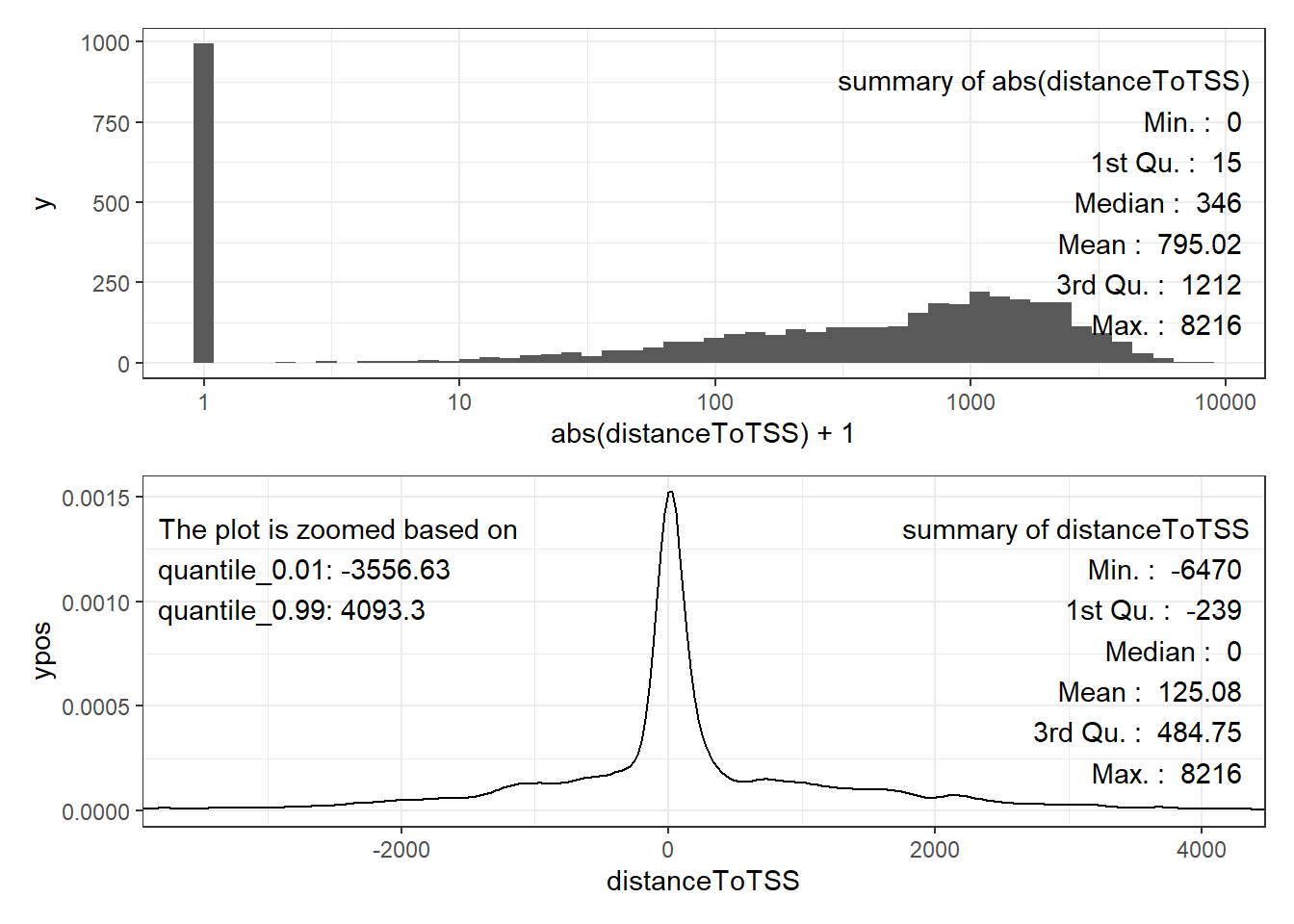
我们可以用Cistrome-GO网页上的人类TF数据做下测试,看下不同类型的TF。
# 加载人类hg38的数据
library(TxDb.Hsapiens.UCSC.hg38.knownGene)
可以看到对于GATA4而言,其主要集中在1e5,即10kb的地方。说明其是一个enhancer类型的TF。那么其衰减距离就可以设置为10kb。
GATA4 <- rtracklayer::import.bed(con = "http://go.cistrome.org/download?uid=1554207232&type=bed&factor=GATA4")

colnames(mcols(GATA4))[1] <- "feature_id"

GATA4
## GRanges object with 14775 ranges and 2 metadata columns:
##           seqnames            ranges strand |  feature_id     score
##              <Rle>         <IRanges>  <Rle> | <character> <numeric>
##       [1]     chr1     629804-630092      * |       peak1  41.75324
##       [2]     chr1     633878-634182      * |       peak2  88.72178
##       [3]     chr1     866046-866210      * |       peak3   8.04482
##       [4]     chr1   1847049-1847308      * |       peak4   6.16494
##       [5]     chr1   2654138-2654347      * |       peak5   6.00395
##       ...      ...               ...    ... .         ...       ...
##   [14771]     chrY 11329763-11330053      * |   peak14771  31.64075
##   [14772]     chrY 11333087-11333349      * |   peak14772  10.82529
##   [14773]     chrY 11721879-11722216      * |   peak14773  31.34938
##   [14774]     chrY 11731167-11731450      * |   peak14774  36.59362
##   [14775]     chrY 56842251-56842525      * |   peak14775   7.68772
##   -------
##   seqinfo: 68 sequences from an unspecified genome; no seqlengths

plot_annoDistance(mm_nearestGene(GATA4, TxDb.Hsapiens.UCSC.hg38.knownGene))
## >> checking seqlevels match...       2021-09-24 16:25:58
## >> your peak_GR seqlevel:chr1 chr10 chr11 chr12 chr13 chr14 chr15 chr16 chr17 chr18...
## >> your Txdb seqlevel:chr1 chr2 chr3 chr4 chr5 chr6 chr7 chr8 chr9 chr10...
## Warning: some peak's Chr is nor in your Txdb, for example: chrGL000008.2 chrGL000195.1 chrGL000205.2 chrGL000214.1 chrGL000216.2 chrGL000219.1 chrGL000220.1 chrGL000224.1 chrGL000225.1 chrKI270330.1...
## I have filtered peaks in these Chr, though seqlevels still retain.
## ------------
## annotating Peak using nearest gene mode begins
## >> preparing gene features information...        2021-09-24 16:25:58
##   228 genes were dropped because they have exons located on both strands
##   of the same reference sequence or on more than one reference sequence,
##   so cannot be represented by a single genomic range.
##   Use 'single.strand.genes.only=FALSE' to get all the genes in a
##   GRangesList object, or use suppressMessages() to suppress this message.
## >> finding nearest gene and calculating distance...      2021-09-24 16:26:00
## >> dealing with gene strand ...      2021-09-24 16:26:00
## >> merging all info together ...     2021-09-24 16:26:00
## >> done      2021-09-24 16:26:00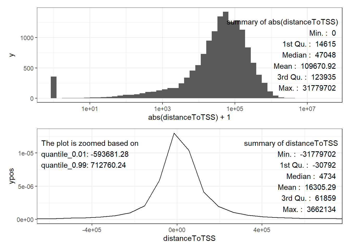
而对于E2F1而言,其主峰还是在0bp那里的,说明其是一个promoter-type的TF。那么其衰减距离就可以设置为1kb。
E2F1 <- rtracklayer::import.bed(con = "http://go.cistrome.org/download?uid=1555419388&type=bed&factor=E2F1")

colnames(mcols(E2F1))[1] <- "feature_id"

E2F1
## GRanges object with 23003 ranges and 2 metadata columns:
##           seqnames            ranges strand |  feature_id     score
##              <Rle>         <IRanges>  <Rle> | <character> <numeric>
##       [1]     chr1     629816-630052      * |       peak1   13.1642
##       [2]     chr1     633907-634162      * |       peak2   25.2659
##       [3]     chr1     778508-779030      * |       peak3   58.9295
##       [4]     chr1     827416-827769      * |       peak4   15.0682
##       [5]     chr1     869736-870026      * |       peak5   50.1306
##       ...      ...               ...    ... .         ...       ...
##   [22999]     chrY 20575445-20575759      * |   peak22999   23.7584
##   [23000]     chrY 56728011-56728279      * |   peak23000   56.7710
##   [23001]     chrY 56734656-56734932      * |   peak23001   62.1793
##   [23002]     chrY 56763385-56763656      * |   peak23002   54.7901
##   [23003]     chrY 56873629-56873923      * |   peak23003   16.0024
##   -------
##   seqinfo: 53 sequences from an unspecified genome; no seqlengths

plot_annoDistance(mm_nearestGene(E2F1, TxDb.Hsapiens.UCSC.hg38.knownGene))
## >> checking seqlevels match...       2021-09-24 16:26:04
## >> your peak_GR seqlevel:chr1 chr10 chr11 chr12 chr13 chr14 chr15 chr16 chr17 chr18...
## >> your Txdb seqlevel:chr1 chr2 chr3 chr4 chr5 chr6 chr7 chr8 chr9 chr10...
## Warning: some peak's Chr is nor in your Txdb, for example: chrGL000009.2 chrGL000194.1 chrGL000195.1 chrGL000205.2 chrGL000216.2 chrGL000218.1 chrGL000219.1 chrGL000220.1 chrGL000225.1 chrKI270333.1...
## I have filtered peaks in these Chr, though seqlevels still retain.
## ------------
## annotating Peak using nearest gene mode begins
## >> preparing gene features information...        2021-09-24 16:26:05
##   228 genes were dropped because they have exons located on both strands
##   of the same reference sequence or on more than one reference sequence,
##   so cannot be represented by a single genomic range.
##   Use 'single.strand.genes.only=FALSE' to get all the genes in a
##   GRangesList object, or use suppressMessages() to suppress this message.
## >> finding nearest gene and calculating distance...      2021-09-24 16:26:06
## >> dealing with gene strand ...      2021-09-24 16:26:06
## >> merging all info together ...     2021-09-24 16:26:06
## >> done      2021-09-24 16:26:06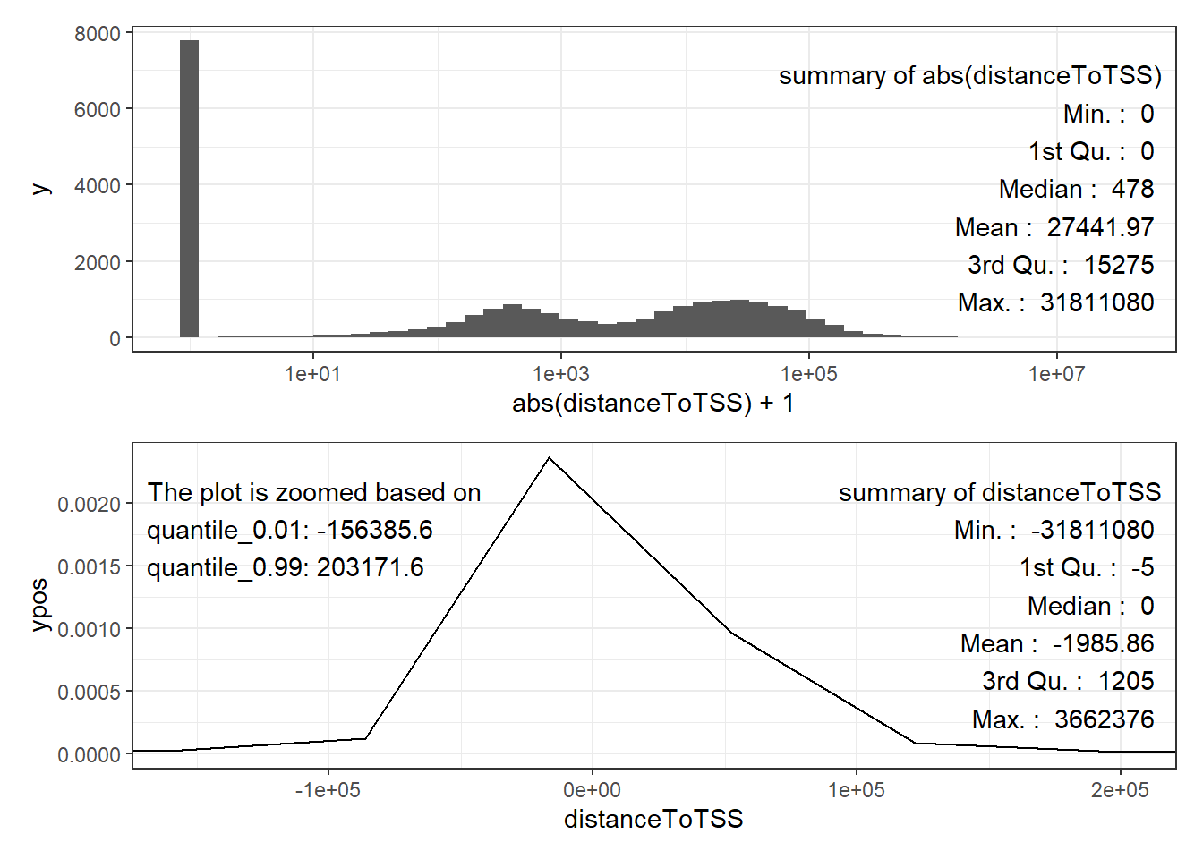
还有就是calcRP_TFHit或者说整个integrate_ChIP_RNA其实借用的是BETA1及其继任者Cistrome-GO2的思想。由于这两个工具都是给人类和小鼠用的,所以作者才自己写了这个模块,来方便其他非模式物种也可以更加准确合理地预测TF target。但是对于那些自身的TF数据是人类或者小鼠的用户来说,我还是推荐使用以上两个工具。因为他们除了用RP以及rank product来提高预测准确率之外,他们还基于自己收集的数据库进行了RP score adjustment。具体一点就是,有某些基因其在大部分的TF ChIP-seq中,都具有很高的RP。但是这些高RP的基因对于预测TF target其实是不利的,因为这些基因可能具有某些管家基因的属性、也有可能是ChIP-seq本底导致的富集,不管怎么样都可以认为是属于TF ChIP-seq的背景。而我们做TF target很多时候是需要你的结果是非常特异的,即只针对你测序的那个TF,所以我们要做RP score adjustment。
RNA-seq rank
RNA-seq的输入格式要求有三列,分别是gene_id, log2FoldChange, padj。这三列也是DESeq2的输出结果,如果你是其他差异分析软件所产生的,可以将对应的列名换成这三列即可。
head(RNADiff_LEC2_GR)
##     gene_id log2FoldChange      padj
## 1 AT5G00730             NA        NA
## 2 AT5G01010    -0.04782798 0.9995524
## 3 AT5G01015    -0.28867596 0.9936103
## 4 AT5G01017             NA        NA
## 5 AT5G01020    -0.13143524 0.9690018
## 6 AT5G01030 -0.30567845 0.2921698RNA-seq的rank非常的简单,就是根据你输入数据中的padj进行排序,padj越小,其排序就在越前面。对于那些padj是NA的基因,其rank就会落到最后面。
integrate_ChIP_RNA
integrate_ChIP_RNA要求你输入的是一个report_fullInfo = FALSE的calcRP_TFHit结果和一个RNA-seq差异分析结果。其最终会综合展现这两者的结果,并给出一个rank product的结果。举个例子就是如果一个基因在TF ChIP-seq中rank是100, 在TF RNA-seq中rank是20,那么其rank product就是
同时还需要注意的是,在integrate_ChIP_RNA函数中还有两个参数,lfc_threshold和padj_threshold。这两个参数的作用并不是决定你最终的TF target预测,而是用来对你的TF type做一个简单的属性预测。
merge_data <- integrate_ChIP_RNA(result_geneRP = TFHit_RP,
                                 result_geneDiff = RNADiff_LEC2_GR,
                                 lfc_threshold = 0.58,
                                 padj_threshold = 0.05)

merge_data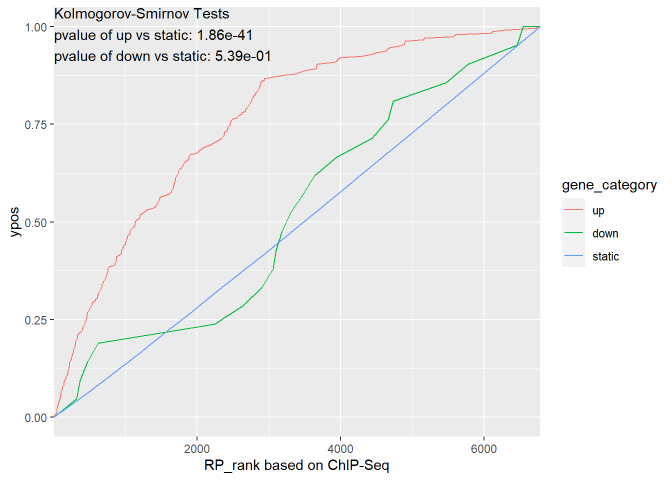
可以看到最终产生的merge_data并不是一个数据框,而是一个ggplot2的对象。他绘制的基本原理是首先根据你设定的lfc_threshold和padj_threshold这两个阈值来确定三个基因集合:上调基因、下调基因和背景基因,即up、down以及static。然后这三个集合中都有各自的RP rank(由calcRP_TFHit计算而来)分布。可以想象,如果你的上调基因集合中,其RP rank都是很靠前的,那么就说明你的TF很有可能起到的是激活作用。不过具体的激活/抑制,还是要看你RNA-seq是OE/KO了。
在得到了三个集合的各自RP分布之后,就可以分别绘制这三个集合的累积分布函数了。假设上调基因集合的RP rank都是很靠前的,占据了1到100,那么可以想象,相比于其他两根曲线,上调基因的累积分布函数很快就会到达1那里,反应到图上面就是其要比其他两根曲线更加地靠上面。这也是我们这个数据集所反应出来的。而对于分布之间的统计检验,我选择了Kolmogorov-Smirnov Tests。如果大家对于三个集合的RP分布感兴趣的话,也可以自己提出来:
category_rank_list <- split(merge_data$data$RP_rank, merge_data$data$gene_category)

str(category_rank_list)
## List of 3
##  $ up    : num [1:241] 23 140 525 200 83 52 62 7 759 43 ...
##  $ down  : num [1:21] 318 366 471 619 2243 ...
## $ static: num [1:6521] 13 1 4 9 2 53 14 3 35 28 ...对于大家最感兴趣的target预测结果,可以直接从merge_data中提取。可以看到,前4列是calcRP_TFHit的结果,随后三列是RNA-seq的结果,然后就是rank product以及rankOf_rankProduct和根据你设定的阈值划分的gene_category。
# 由于tibble对象无法展示全部column,我将其转变成了data.frame
# 正常提取可以用merge_data$data
head(as.data.frame(merge_data$data))
##     gene_id withPeakN    sumRP RP_rank log2FoldChange          padj diff_rank
## 1 AT5G23370         9 2.842045      23       3.557105  2.329837e-46        12
## 2 AT5G13910        11 2.298318     140       4.204242  1.360894e-85         2
## 3 AT5G23350        10 1.675591     525       3.199794 1.338479e-121         1
## 4 AT5G23360        10 2.121829     200       2.985809  2.243615e-64         6
## 5 AT5G52882        17 2.498138      83       1.631654  1.927703e-36        15
## 6 AT5G05180        21 2.611409      52       1.219398  3.576526e-23        27
##   rankProduct rankOf_rankProduct gene_category
## 1         276                  1            up
## 2         280                  2            up
## 3         525                  3            up
## 4        1200                  4            up
## 5        1245                  5            up
## 6        1404                  6            up
需要注意的是,尽管用这RP和rank product的方式来预测靶基因会比单纯地用最近基因注释加阈值筛选更加的合理。但也会带来一个“坏处”,即它不能立刻带给你一个gene list,同时由于RP是gene TSS scan 10kb甚至100kb的结果,那些RP很低的基因也会考虑在内。最后的数据集可能会有上w的基因,但对于大部分的TF来说,不太可能存在几w的target gene。所以这其中肯定会有一些噪音。这时候除了武断地挑选前1000或者前5000基因之外,可以考虑基于一些已知的靶基因,看看其对应的rank值,从而来确定target gene的rank下界。
Reference
Wang, S., Sun, H., Ma, J., Zang, C., Wang, C., Wang, J., Tang, Q., Meyer, C.A., Zhang, Y., and Liu, X.S. (2013). Target analysis by integration of transcriptome and ChIP-seq data with BETA. Nat Protoc 8, 2502–2515.↩︎
Li, S., Wan, C., Zheng, R., Fan, J., Dong, X., Meyer, C.A., and Liu, X.S. (2019). Cistrome-GO: a web server for functional enrichment analysis of transcription factor ChIP-seq peaks. Nucleic Acids Research 47, W206–W211.↩︎
Guandong Shang
PhD Candidate
My research interests include rstats, epigenomics, bioinformatics and evo-devo.